Splining#
This section gives an in-depth overview of the steps taken in the splining module.
At a Glance : Smoothing Pixelated Traces#
The splining.py module handles all the functions associated with smoothing the ordered pixel-wise trace from the
“ordered_tracing” step, in order to produce curves which more closely follow the samples structure.
The quality of the resultant metrics and smoothed coordinates will depend on the splining method chosen, whether the ordering worked successfully, and whether the skeleton matches the underlying sample conformation.
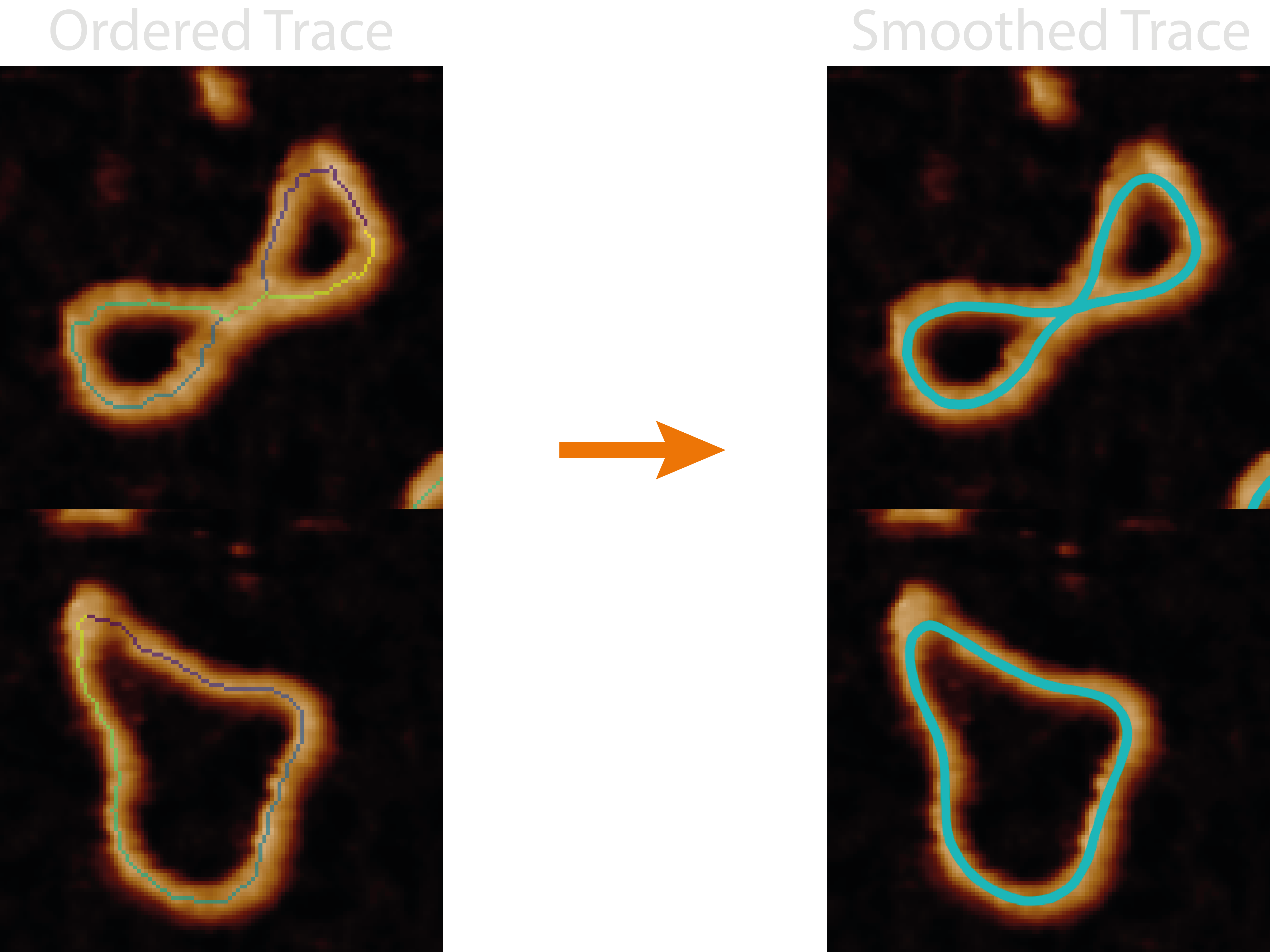
This smooths the ordered trace by using an average of splines through the ordered coordinates (spline method) or using
the mean coordinate of a rolling window (rolling_window method), helping to resolve length errors in jagged in the
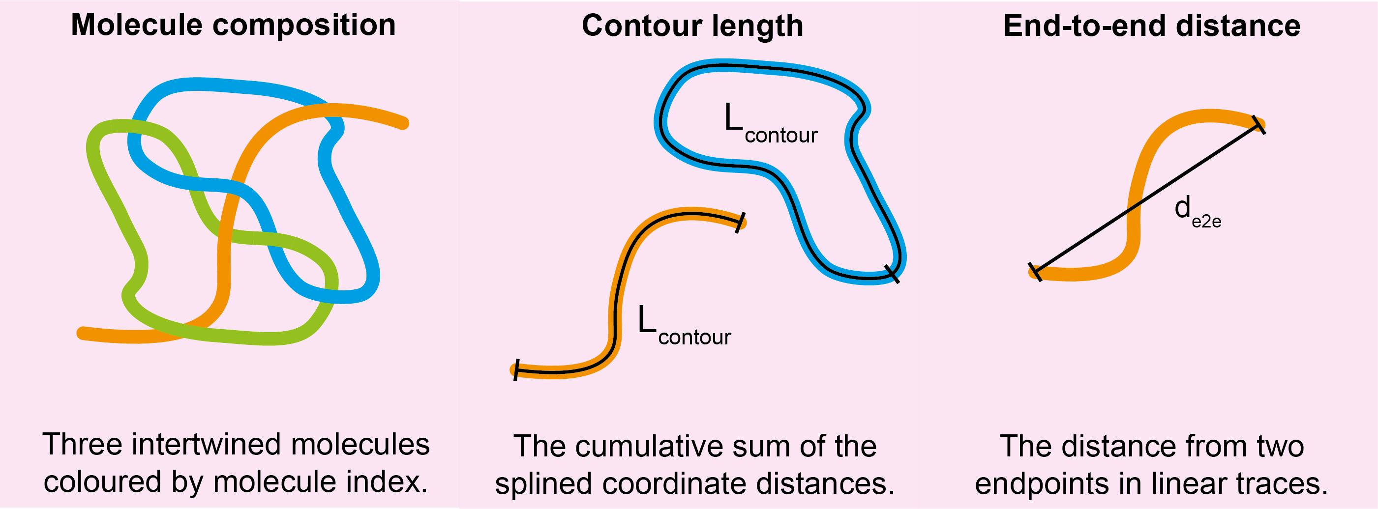
skeletons. It adds the contour length and end-to-end euclidean distance to the molecule_statistics.csv and the sum and
average of these respectively to the grain_statistics.csv.
Some quick FYI’s:
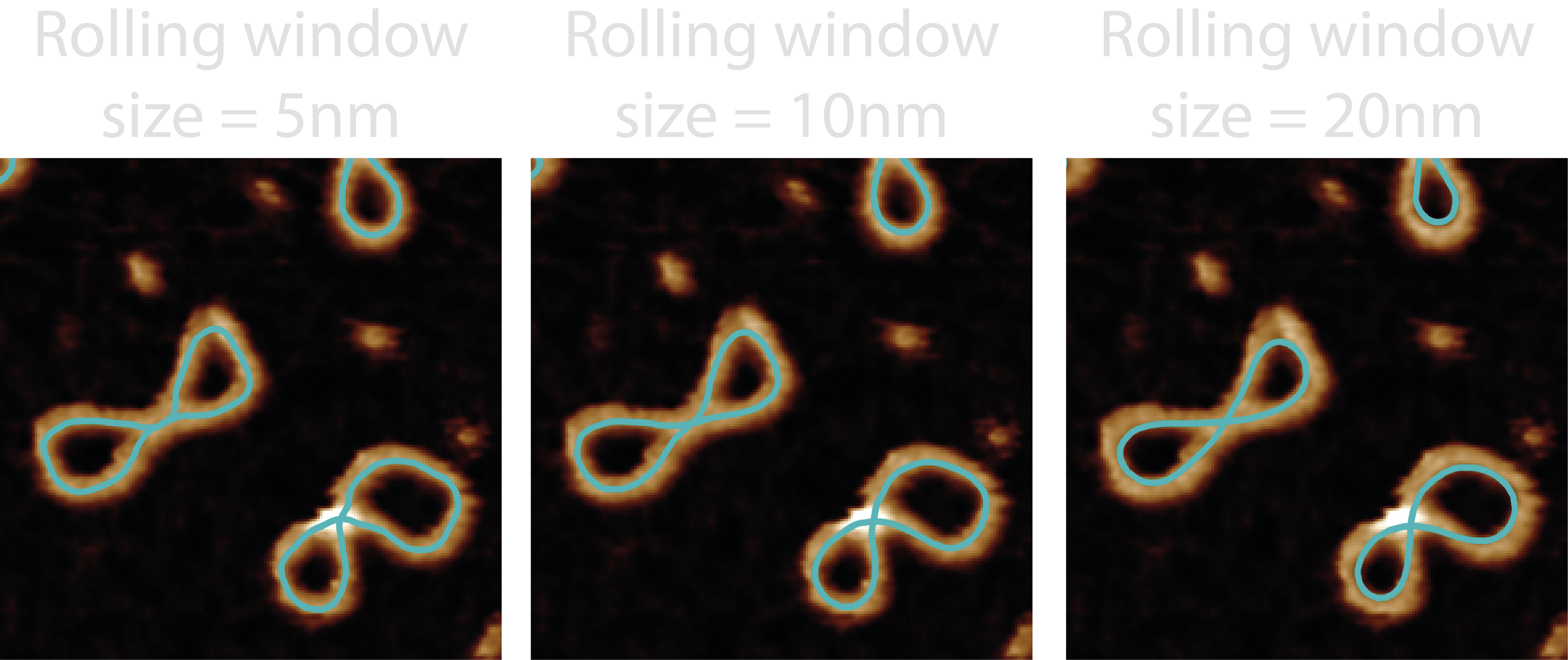
Constricted Traces - Using the
rolling_windowmethod with a rolling window size that is not far below the persistence length can result in over-smoothing where the spline is dragged away from regions of high curvature.Unrepresentative Splines - The
splinemethod’s parameters can be quite temperamental so it’s recommended thatspline_linear_smoothing,spline_circular_smoothingandspline_degreeare not changed unless understood.Unrepresentative Splines 2 - The
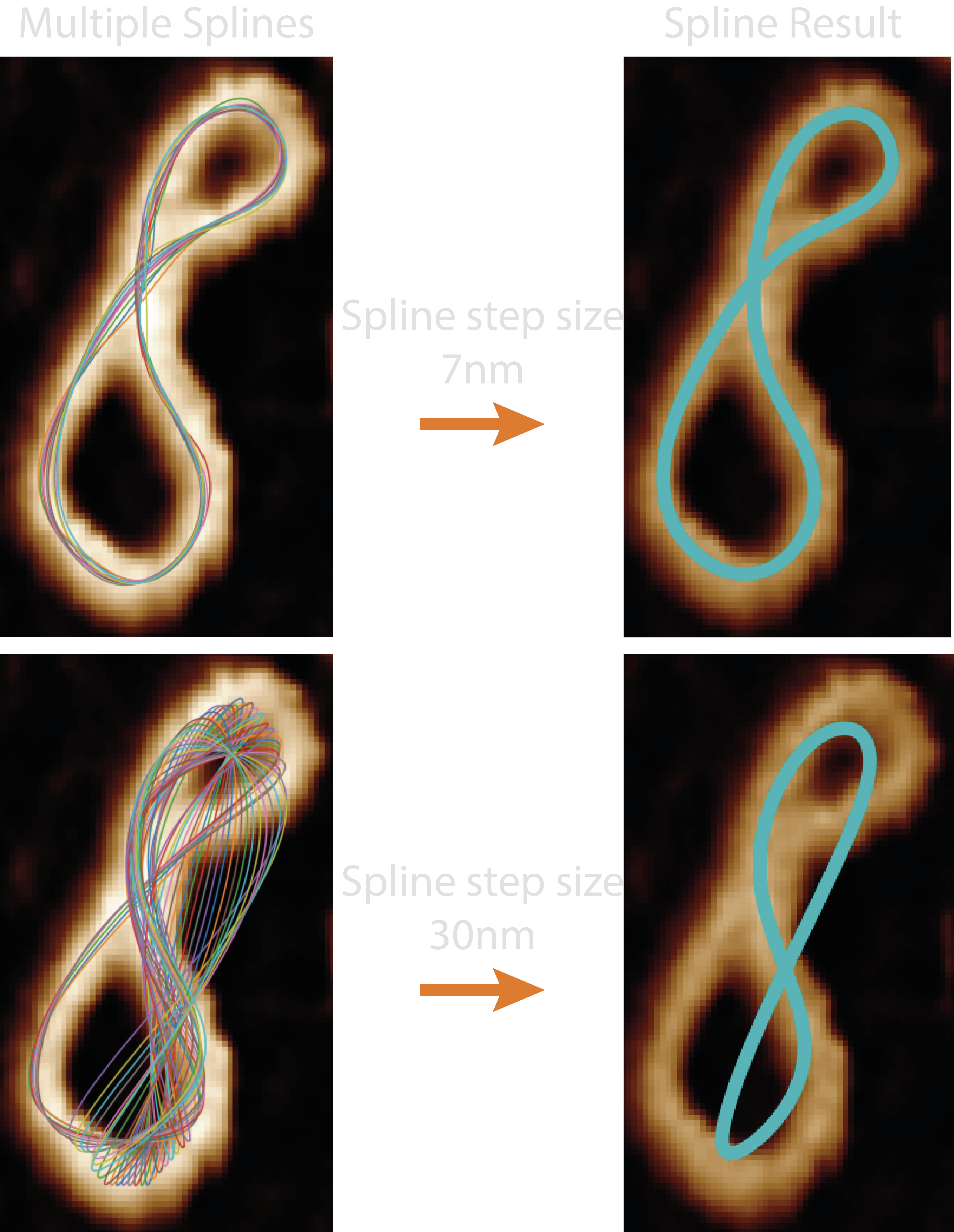
splinemethod may produce unwanted results if thespline_step_sizeis too long. This is because the way the splines are averaged assumes that each spline point is sampled close to that of another’s.
Processing Steps#
Splining Method#
1. Trace Coordinate Subsets#
The first stage is to use the ordered coordinates and the spline_step_size parameter to define how many splines we
want to average together. As the spline_step_size is the distance (in nm) at which to take every i’th coordinate for
its spline. This means the number of splines to average is calculated below:
$$ N = max(\text{spline step size} \div \text{px to nm}, 1) $$
The coordinates used for each spline are then obtained from the initial ordered trace, i.e. the spline coordinate indexes: [1, 2, 3, 4, 1, 2, 3, 4, 1, 2, 3, 4], where spline 1 takes every 4th coordinate, starting at position 0, then spline 2 takes every 4th coordinate starting at position 1, etc.
2. Obtaining Splines#
For each of these coordinate subsets, we use the
Sci-Py
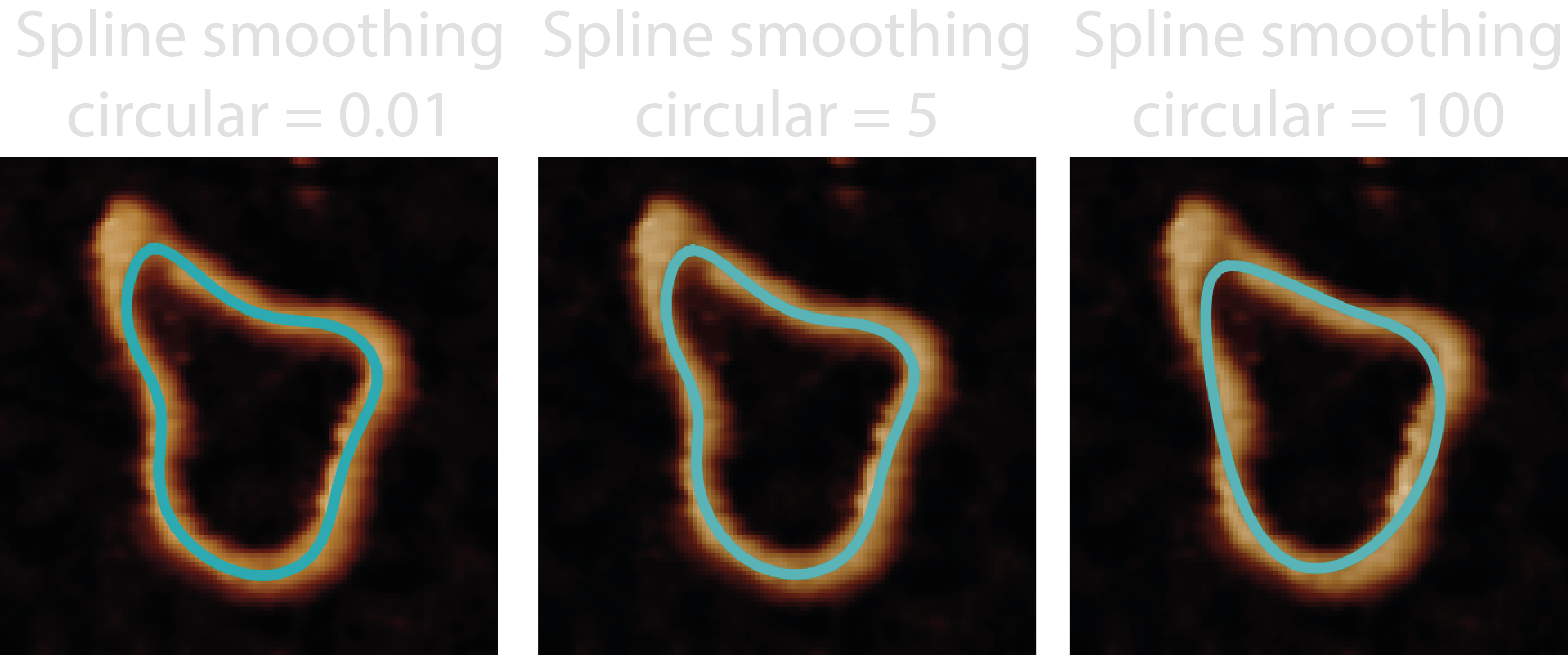
library to find the B-Spline representation of the 2D curve using the smoothness parameters spline_linear_smoothing,
spline_circular_smoothing, and the spline_degree, found in the configuration file. The spline_linear_smoothing and
spline_circular_smoothing define the degrees of smoothing for circular or linear molecules obtained in the Ordered
Tracing step, which also tells TopoStats whether to make the spline periodic if circular. Larger smoothing values mean
more smoothing and smaller values indicate less smoothing. The spline_degree should take odd values, or even with
large smoothing. Read more on the Sci-Py documentation above.
These splines are then averaged together via their index i.e. first spline coordinates are averaged, then second
etc… until a single averaged B-Spline remain. However, because the splined are averaged on their index, it is assumed
that each index is within close proximity, thus, the spline_step_size must be small enough for this assumption to hold
true and for the splining to work as intended.
Rolling Window Method#
1. Rolling Average#
This method simply uses a rolling average of the ordered trace coordinates within the rolling_window_size to produce
the new smoothed trace. The rolling window will move one coordinate along each time, and continues until the start of
the window returns back to its initial position.
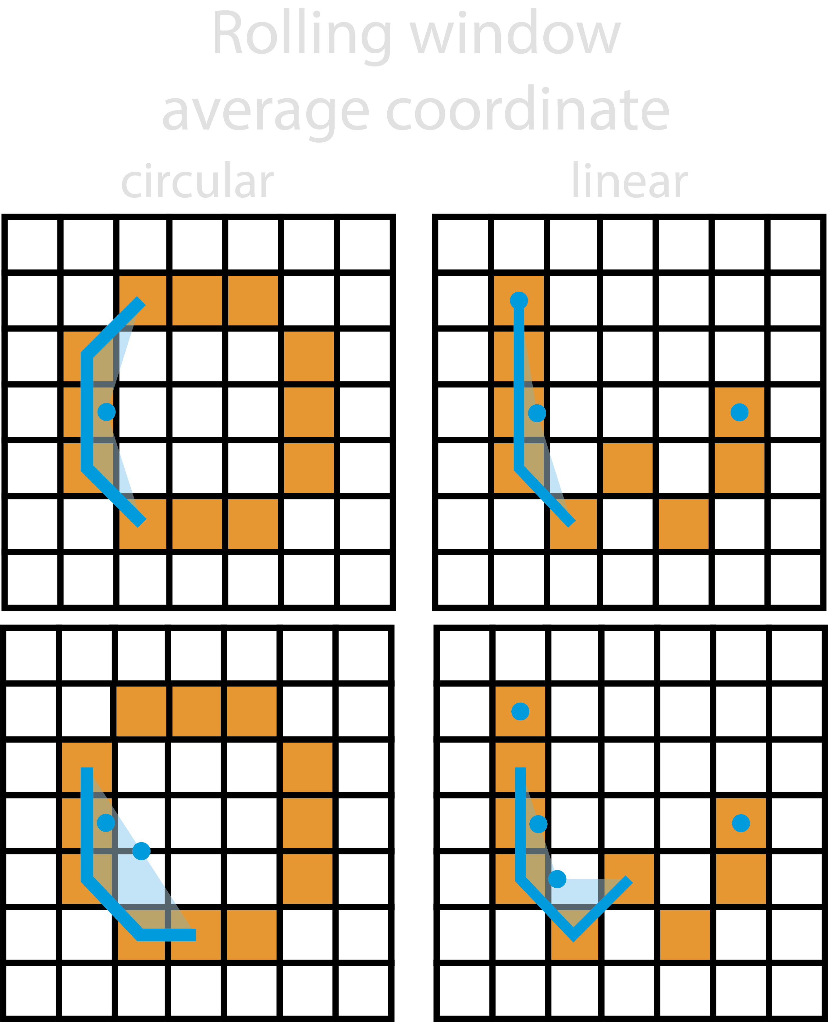
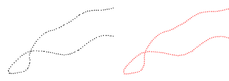
For linear smooth traces, the same as above occurs however, the initial and final coordinates are also added to the smoothed trace as to not drastically reduce the length of the smoothed trace.
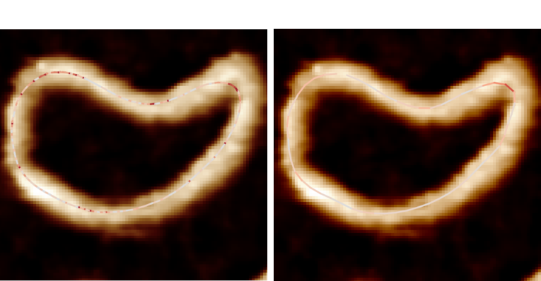
Resampling#
As an optional extra step in the rolling window method, the smoothed coordinates can be resampled to a set of coordinates that are evenly spaced in space, ie each coordinate is say 1nm apart. This is not the same as interpolation as interpolation is not guaranteed to be evenly spaced.
Using resampling can make the results of curvature measurements more representative of the actual curvature of the trace.
Outputs#
The <image>_<threshold>_ordered_traces image shows the direction of ordered coordinates.
For each grain, the following new columns are added to the grainstats.csv file:
| Column Name | Description | Data Type |
|---|---|---|
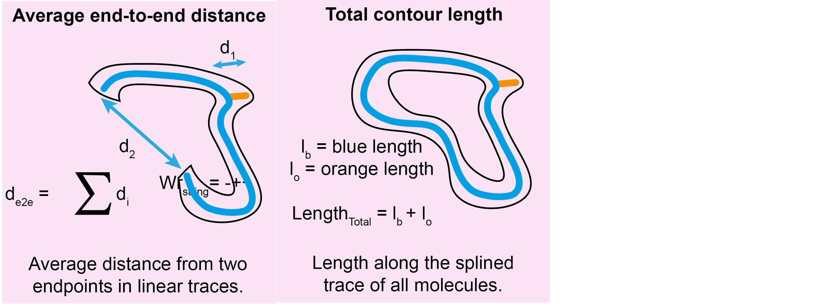
total_contour_length |
The total length along the splined trace of all identified molecules. | float |
average_end_to_end_distance |
The average distance from two endpoints of the spline of all identified linear molecules. | float |
For each molecule found by the ordering algorithm(s), the following new columns are added to the molstats.csv file:
| Column Name | Description | Data Type |
|---|---|---|
contour_length |
The length along the splined trace of the molecule. | float |
end_to_end_distance |
The distance from two endpoints of the spline of the linear molecule. | float |
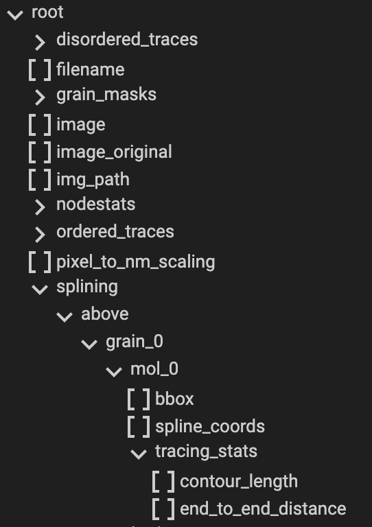
Note: Most information obtained during the Splining processing can be obtained from the <image_name>.topostats file
found within the processed folder and contains a multitude of molecule related objects such as:
bounding box
spline coordinates
tracing statistics of contour length and end to end distance
Diagnostic Images#
There are no diagnostic images produced in this step.
Possible Uses#
This module would lend itself useful for accurately measuring the lengths of complex objects within samples, and obtaining an accurate representation of the underlying conformation of the sample.
We have used this module to accurately measure the length of topologically complex DNA samples such as knots, catenanes, and theata-curves (replication intermediates). Additionally, we’ve used the end-to-end distance to measure the conformational variation of linear DNA in the presence of NDP-52 to show that it may also play a role in topological regulation. See more here..